43 adding labels to excel chart
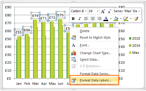
Add label to Excel chart line - AuditExcel.co.za Adding a label to an Excel line chart is very easy. As shown below, you can create the chart and then right click on the line and choose 'Add Data Labels' and then 'Add Data Labels' again. The labels are immediately put on the chart and Excel has 'guessed' that you wanted the values to appear. Adding rich data labels to charts in Excel 2013 | Microsoft 365 Blog One familiar and simple way is just single click on any data value (or column, in this example) to select the entire data series that it belongs to. Above, I have clicked all of the blue columns. Once the series is selected, I can right-click any column to pull up the context menu, then click the Add Data Labels entry.
Comparison Chart in Excel | Adding Multiple Series Under Same … Guide to Comparison Chart in Excel . ... Just make sure the names you are adding for the chart title and axis title are relevant to your chart data. Usually, chart headers are used as axis labels/titles. This is how we can configure Comparison Chart under Excel. Let’s wrap things up with some points to be remembered.

Adding labels to excel chart
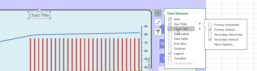
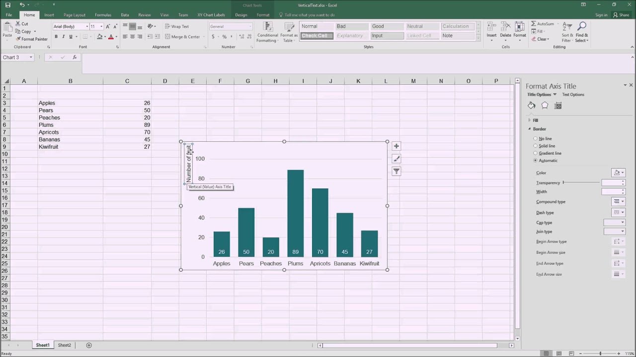
How to Add Axis Labels in Excel Charts - Step-by-Step (2022) - Spreadsheeto How to add axis titles 1. Left-click the Excel chart. 2. Click the plus button in the upper right corner of the chart. 3. Click Axis Titles to put a checkmark in the axis title checkbox. This will display axis titles. 4. Click the added axis title text box to write your axis label. Data Labels in Excel Pivot Chart (Detailed Analysis) Add a Pivot Chart from the PivotTable Analyze tab. Then press on the Plus right next to the Chart. Next open Format Data Labels by pressing the More options in the Data Labels. Then on the side panel, click on the Value From Cells. Next, in the dialog box, Select D5:D11, and click OK. How to Insert Axis Labels In An Excel Chart | Excelchat We will go to Chart Design and select Add Chart Element Figure 6 - Insert axis labels in Excel In the drop-down menu, we will click on Axis Titles, and subsequently, select Primary vertical Figure 7 - Edit vertical axis labels in Excel Now, we can enter the name we want for the primary vertical axis label.
Adding labels to excel chart. Adding Colored Regions to Excel Charts - Duke Libraries Center … 12-11-2012 · Time series data is easy to display as a line chart, but drawing an interesting story out of the data may be difficult without additional description or clever labeling. One option, however, is to add regions to your time series charts to indicate historical periods or visualization binary data. Here is an example where a … Continue reading Adding Colored Regions to … How to Add Data Labels in Excel - Excelchat | Excelchat After inserting a chart in Excel 2010 and earlier versions we need to do the followings to add data labels to the chart; Click inside the chart area to display the Chart Tools. Figure 2. Chart Tools Click on Layout tab of the Chart Tools. In Labels group, click on Data Labels and select the position to add labels to the chart. Figure 3. Adding Data Labels to Charts/Graphs in Excel - AdvantEdge Training ... First Method - In the Design tab of the Chart Tools contextual tab, go to the Chart Layouts group on the far left side of the ribbon, and click Add Chart Element. In the drop-down menu, hover on Data Labels. This will cause a second drop-down menu to appear. Choose Outside End for now and note how it adds labels to the end of each pie portion. How to add or move data labels in Excel chart? - ExtendOffice To add or move data labels in a chart, you can do as below steps: In Excel 2013 or 2016. 1. Click the chart to show the Chart Elements button .. 2. Then click the Chart Elements, and check Data Labels, then you can click the arrow to choose an option about the data labels in the sub menu.See screenshot:
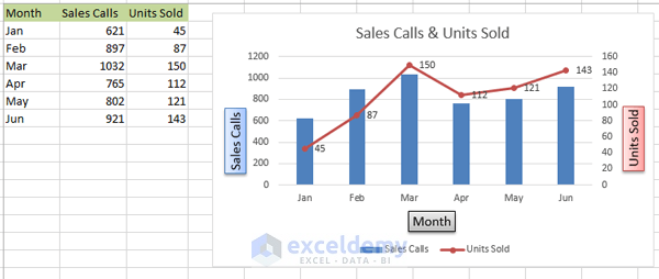
How to Use Cell Values for Excel Chart Labels - How-To Geek Select the chart, choose the "Chart Elements" option, click the "Data Labels" arrow, and then "More Options." Uncheck the "Value" box and check the "Value From Cells" box. Select cells C2:C6 to use for the data label range and then click the "OK" button. The values from these cells are now used for the chart data labels. how to add data labels into Excel graphs - storytelling with data To adjust the number formatting, navigate back to the Format Data Label menu and scroll to the Number section at the bottom. I'll choose Number in the Category drop-down and change Decimal places to 0 (side note: checking the Linked to source box is a good option if you want the labels to reformat when the formatting of the underlying source data changes). How to Add Data Labels to an Excel 2010 Chart - dummies Select where you want the data label to be placed. Data labels added to a chart with a placement of Outside End. On the Chart Tools Layout tab, click Data Labels→More Data Label Options. The Format Data Labels dialog box appears. How to Make a Pie Chart in Excel (Only Guide You Need) 13-07-2022 · Read More: How to Make Pie Chart in Excel with Subcategories (2 Quick Methods) Conclusion. Hope after reading this article you will not face any difficulties with the pie chart. This article covers all the necessary things regarding Excel Pie Chart. Stay tuned for more useful articles. Let us know what problems do you face with Excel Pie Chart.
How to Change Excel Chart Data Labels to Custom Values? 05-05-2010 · We all know that Chart Data Labels help us highlight important data points. When you "add data labels" to a chart series, excel can show either "category" , "series" or "data point values" as data labels. But what if you want to have a data label show a different value that one in chart's source data? Use this tip to do that. Dynamically Label Excel Chart Series Lines - My Online Training … 26-09-2017 · Hi Mynda – thanks for all your columns. You can use the Quick Layout function in Excel (Design tab of the chart) to do the labels to the right of the lines in the chart. Use Quick Layout 6. You may need to swap the columns and rows in your data for it to show. Then you simply modify the labels to show only the series name. How to Show Percentage in Excel Pie Chart (3 Ways) 03-07-2022 · 2. Display Percentage in Pie Chart by Using Format Data Labels. Another way of showing percentages in a pie chart is to use the Format Data Labels option.We can open the Format Data Labels window in the following two ways.. 2.1 Using Chart Elements. To active the Format Data Labels window, follow the simple steps below.. Steps: Edit titles or data labels in a chart - support.microsoft.com On a chart, click the label that you want to link to a corresponding worksheet cell. On the worksheet, click in the formula bar, and then type an equal sign (=). Select the worksheet cell that contains the data or text that you want to display in your chart. You can also type the reference to the worksheet cell in the formula bar.
Charting in Excel - Adding Data Labels - YouTube
Add or remove data labels in a chart - support.microsoft.com Tip: You can use either method to enter percentages — manually if you know what they are, or by linking to percentages on the worksheet.Percentages are not calculated in the chart, but you can calculate percentages on the worksheet by using the equation amount / total = percentage.For example, if you calculate 10 / 100 = 0.1, and then format 0.1 as a percentage, the number will …

Lesson 2 | How to Create Charts Using Microsoft Excel Tutorial
Excel: How to Create a Bubble Chart with Labels - Statology To add labels to the bubble chart, click anywhere on the chart and then click the green plus "+" sign in the top right corner. Then click the arrow next to Data Labels and then click More Options in the dropdown menu: In the panel that appears on the right side of the screen, check the box next to Value From Cells within the Label Options ...
Add a label and other information to axes in a Graph or Chart in Excel by Excel Made Easy
How to Insert Axis Labels In An Excel Chart | Excelchat We have a sample chart as shown below; Figure 2 – Adding Excel axis labels. Next, we will click on the chart to turn on the Chart Design tab; We will go to Chart Design and select Add Chart Element; Figure 3 – How to label axes in Excel . In the drop-down menu, we will click on Axis Titles, and subsequently, select Primary Horizontal Figure ...
Excel Custom Chart Labels • My Online Training Hub
Labels - How to add labels | Excel E-Maps Tutorial You can add a label to a point by selecting a column in the LabelColumn menu. Here you can see an example of the placed labels. If you would like different colors on different points you should create a thematic layer. You can do this by following the tutorial about Thematic Points and to chooce Individual Colors. You can find the tutorial here.
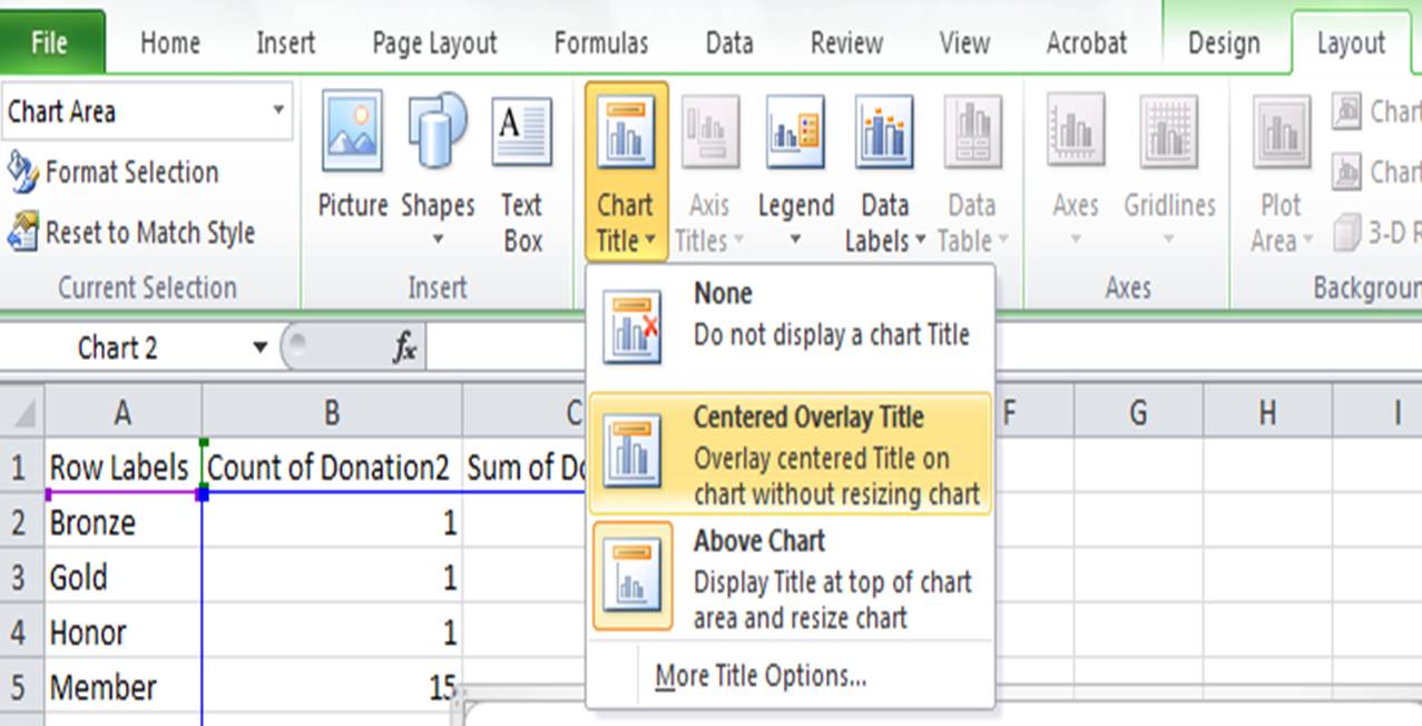
Excel Chart Options: Adding Titles | Pryor Learning Solutions
Data Labels disappearing off excel chart | MrExcel Message Board When I right click on the data label and click format data label, I go down to Number where it is defaulted to General under format code and linked to source is ticked. Instead of showing $150,000,000 I want it to show $150.0m so I edit the format code box to $0.0,,"m" and click add. The format code box changes to the formula I entered but the ...

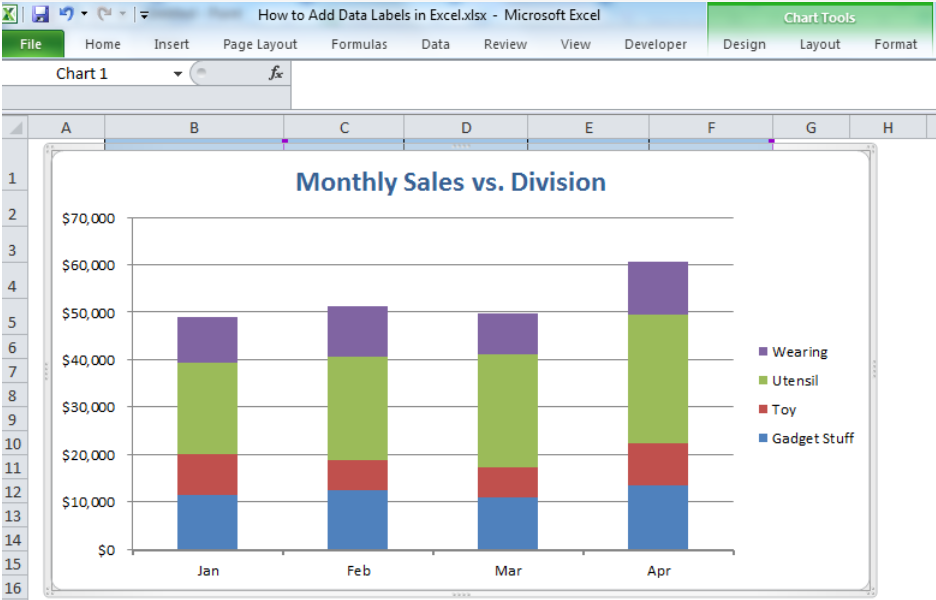
How to add total labels to stacked column chart in Excel?
How to add axis label to chart in Excel? - ExtendOffice Select the chart that you want to add axis label. 2. Navigate to Chart Tools Layout tab, and then click Axis Titles, see screenshot: 3.

10 Design Tips to Create Beautiful Excel Charts and Graphs in 2017
How to Add Labels to Scatterplot Points in Excel - Statology Step 3: Add Labels to Points Next, click anywhere on the chart until a green plus (+) sign appears in the top right corner. Then click Data Labels, then click More Options… In the Format Data Labels window that appears on the right of the screen, uncheck the box next to Y Value and check the box next to Value From Cells.
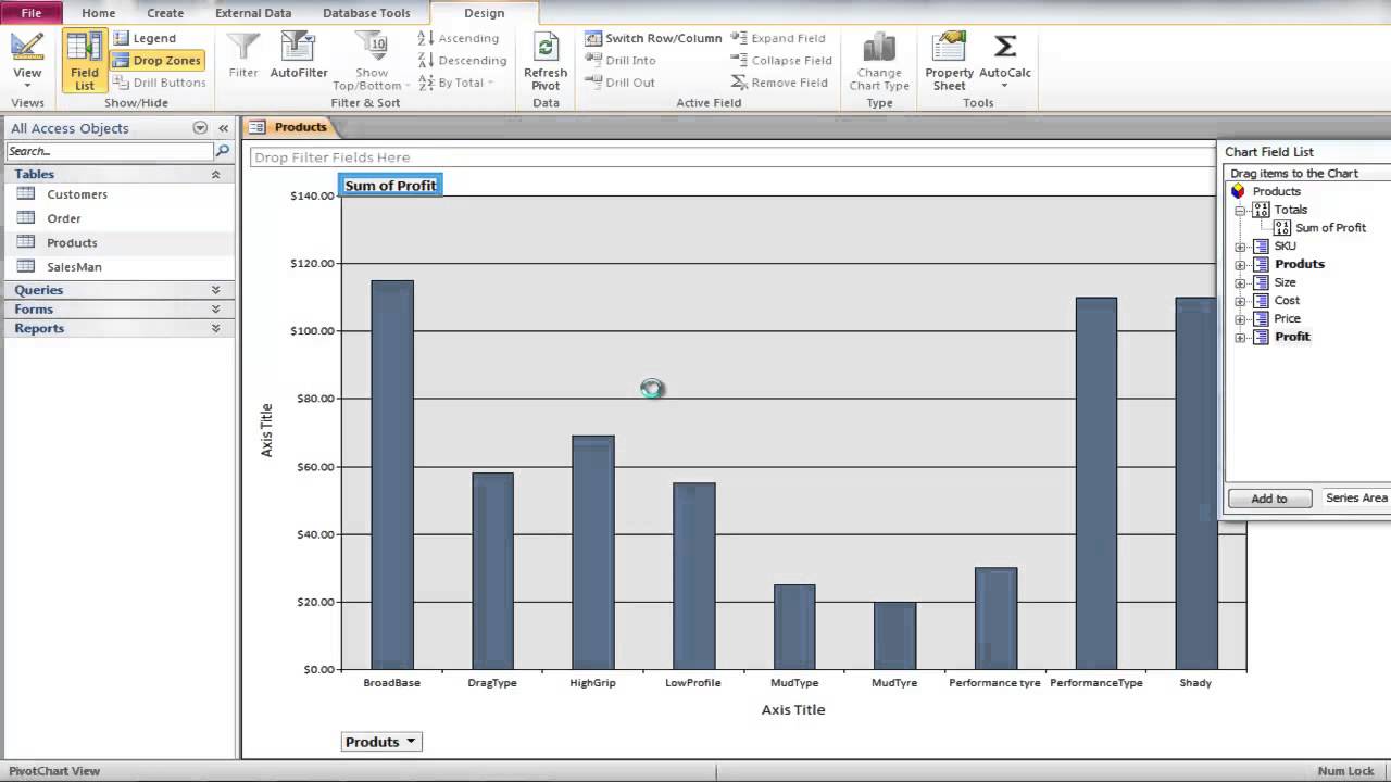
How to Create a Pivot Chart in Microsoft Access - YouTube
How to Add Axis Labels to a Chart in Excel | CustomGuide Add Data Labels. Use data labels to label the values of individual chart elements. Select the chart. Click the Chart Elements button. Click the Data Labels check box. In the Chart Elements menu, click the Data Labels list arrow to change the position of the data labels.
How to Add Data Labels in Excel - Excelchat | Excelchat
Percentage Change Chart – Excel – Automate Excel This tutorial will demonstrate how to create a Percentage Change Chart in all versions of Excel. Percentage Change – Free Template Download Download our free Percentage Template for Excel. Download Now Percentage Change Chart – Excel Starting with your Graph In this example, we’ll start with the graph that shows Revenue for the last 6…
Creating a chart with dynamic labels - Microsoft Excel 2013
Adding Data Labels To An Excel Chart | MyExcelOnline In our example below, I add a Data Label to a column chart and then I format the data label using CTRL+1. I then select to custom format the numbers so it shows the values as thousands by adding a comma , after each zero and then showing the work k by adding "k" Example Custom Number Format: [$$-1004]#,##0 ,"k" ;- [$$-1004]#,##0 ,"k"

Excel Custom Chart Labels • My Online Training Hub
How to add axis label to chart in Excel? - tutorialspoint.com Now, select the chart for which you want to insert an axis label by clicking. Step 5. Click on the Chart Elements (+) button next to the chart. Then, in the upper-right corner of the chart, click the Chart Elements (+) button. Check the Axis Titles option in the enlarged menu, as seen in the below screenshot.
Excel Chart Elements: Parts of Charts in Excel | ExcelDemy
How to display leader lines in pie chart in Excel? - ExtendOffice 1. Click at the chart, and right click to select Format Data Labels from context menu. 2. In the popping Format Data Labels dialog/pane, check Show Leader Lines in the Label Options section. See screenshot: 3. Close the dialog, now you can see some leader lines appear. If you want to show all leader lines, just drag the labels out of the pie ...

One click to add total label to stacked chart in Excel
How to Add Axis Labels to a Chart in Excel Step 1: Click on a blank area of the chart. Use the cursor to click on a blank area on your chart. Make sure to click on a blank area in the chart. The border around the entire chart will become highlighted. Once you see the border appear around the chart, then you know the chart editing features are enabled.

How to add total labels to stacked column chart in Excel?
Add / Move Data Labels in Charts - Excel & Google Sheets Adding Data Labels Click on the graph Select + Sign in the top right of the graph Check Data Labels Change Position of Data Labels Click on the arrow next to Data Labels to change the position of where the labels are in relation to the bar chart Final Graph with Data Labels
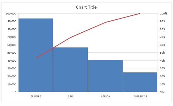
Create a Pareto Chart With Excel 2016 | Free Microsoft Excel Tutorials
Add a DATA LABEL to ONE POINT on a chart in Excel All the data points will be highlighted. Click again on the single point that you want to add a data label to. Right-click and select ' Add data label '. This is the key step! Right-click again on the data point itself (not the label) and select ' Format data label '. You can now configure the label as required — select the content of ...
Adding horizontally-aligned y-axis titles to charts in Excel 2016 - YouTube
Add or remove data labels in a chart - support.microsoft.com Add data labels to a chart Click the data series or chart. To label one data point, after clicking the series, click that data point. In the upper right corner, next to the chart, click Add Chart Element > Data Labels. To change the location, click the arrow, and choose an option.

32 Excel Chart Add Label - Labels Design Ideas 2020
Excel charts: add title, customize chart axis, legend and data labels Click the Chart Elements button, and select the Data Labels option. For example, this is how we can add labels to one of the data series in our Excel chart: For specific chart types, such as pie chart, you can also choose the labels location. For this, click the arrow next to Data Labels, and choose the option you want.
Post a Comment for "43 adding labels to excel chart"